KDB.AI’s Temporal Similarity Search (TSS) provides a comprehensive suite of tools for analyzing patterns, trends, and anomalies within time series datasets. TSS consists of two key components: Transformed and Non-Transformed. Transformed TSS specializes in highly efficient vector searches across massive time series datasets such as historical or reference datasets. Non-Transformed TSS performs near real-time similarity search on fast-moving time series data. With TSS, all of your time series data can be searched and analyzed faster and more efficiently than ever.
Transformed Temporal Similarity Search
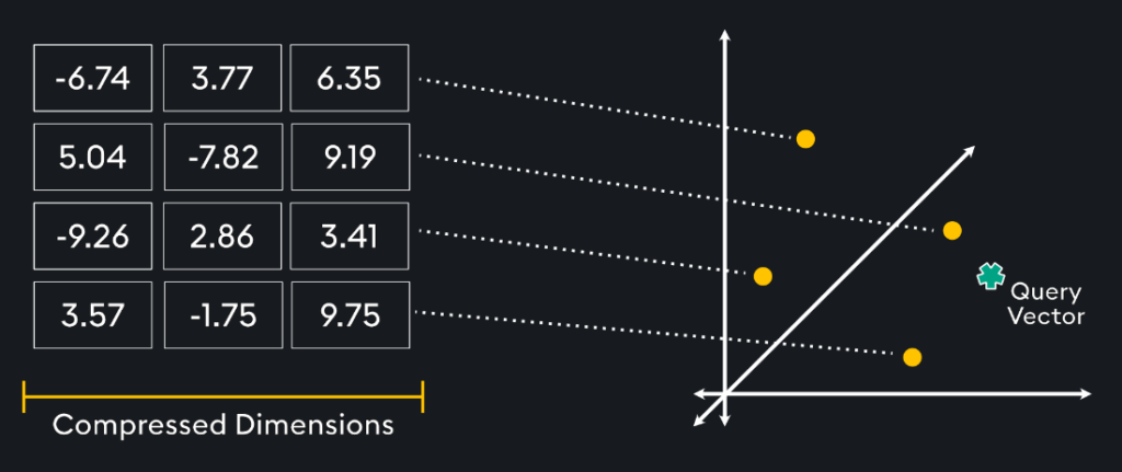
Transformed Temporal Similarity Search is our patent-pending compression model designed to dimensionally reduce time series windows by more than 99%. With Transformed Temporal Similarity Search, KDB.AI can compress times series windows containing thousands of data points, into significantly smaller dimensions, all while maintaining the integrity of the original data’s shape. These compressed windows are then stored within KDB.AI as vector embeddings, setting up the ability to execute vector searches and enabling the efficient analysis of time series datasets.
Flexible Compression Across Varying Sample Rates
Another remarkable capability lies in its ability to compress windows of identical time frames, that contain different numbers of data points, into the same dimensionality. This flexibility enables the handling of time series data with varying sample rates. Ensure that the windows being searched for, and the windows being searched over are for the same time frame.
Transformed TSS Supports ANN Indexing
Transformed Temporal Similarity Search can attach compressed embeddings to prebuilt indexes in the vector database. By attaching the compressed time series vector embeddings to an approximate nearest neighbor (ANN) index, such as Hierarchical Navigable Small World (HNSW), developers can expect to see significantly boosted similarity search speed and performance. Attaching embeddings to an index is particularly beneficial to enhance processing speed when working with large numbers of vector embeddings.
The Proof is in the Performance
By reducing the dimensionality of time-series data streams, Transformed Temporal Similarity Search achieves several benefits:
- Memory and Disk Savings: Transformed Temporal Similarity Search significantly reduces memory usage and disk space requirements. This efficiency translates to better resource utilization and cost savings.
- Optimized Vector Search: When performing vector searches, Transformed TSS minimizes the computational burden. Fewer operations are needed to calculate distance metrics, resulting in faster and more efficient queries.
For a practical illustration, consider this notebook available on GitHub. In this specific scenario a 1000-point time series window is reduced to just 8 dimensions:
- On-Disk & In-Memory performance is greatly increased due to ~100x space savings.
- Insertion of compressed time-series vectors improves by a factor of 2, search speed accelerates by a factor of 10x.
Transformed Temporal Similarity Search Implementation
To create a table in KDB.AI capable of Transformed Temporal Similarity Search, we must add an embedding of type “tsc” to the index column. See the technical documentation here for a deep dive on implementation.
schema = [
        {
            "name":'index',
            "type":'int64'
        },
        {
            "name":'sym',
            "type":'str'
        },
        {
            "name":'time',
            "type":'datetime64[ns]'
        },
        {
            "name":'price',
            "type":'float64s'
        }
      ]

# Define the index
indexes = [
  {
      'type': 'flat',
      'name': 'flat_index',
      'column': 'price',
      'params': {'metric': "L2"},
  },
]

# Define an embedding configuration, specifying to use 'TSC': transformed TSS
# Inserted high dimensional data will be compressed with 'tsc' to 8 dimensions and stored in KDB.AI
embedding_configuration = {'price':{"dims":8, "type":"tsc", "on_insert_error": "reject_all"}}

# Create the table with the defined schema, index, and embedding configuration from above
table = db.create_table(
    table='trade_tsc',
    schema=schema,
    indexes=indexes,
    embedding_configuration=embedding_configuration
)
In this example schema, we define several metadata columns including “index”, “sym”, and “time”. We also define a “price” column that will execute transformed Temporal Similarity Search on time series windows. Next, we define the indexes and embedding configuration, let’s dive into this deeper:
- indexes: holds information on the index, search metric, and vector dimensions
- type: flat, the index type
- name: A user defined name for the index
- column: The column in the schema that this index will be applied to
- params: Holds additional information like the distance metric, L2 (Euclidean Distance), could also be Dot Product or Cosine Similarity.
- embedding_configuration: Key that holds the configuration compressed vectors.
- dims: The dimension after compression.
- type: “tsc”, the embedding method to use, ‘tsc’ is for Transformed Temporal Similarity Search.
- on_insert_error: reject_all, response to errors on insertion.
Use Cases
- Financial and Market Predictions: Financial analysts can use Transformed Temporal Similarity Search to analyze early market data indicators against comprehensive historical archives. This helps steer market forecasts and enrich predictive machine learning models.
- Marketing Optimization: Transformed Temporal Similarity Search can also assist in the analysis of user interaction data, such as clicks, views, and duration to uncover concealed patterns and trends. By forecasting behavior, companies can determine the best times and situations for ad campaigns that boost impact and engagement.
- Retail: Applying a similar concept to the retail industry, Transformed Temporal Similarity Search enhances analysis of customer buying behaviors. Retailers can now segment purchase history data into time windows and process them using KDB.AI. This results in advanced similarity searches that unveil subtle purchase patterns, detect seasonal variations, and track evolving consumer preferences.
Technical Considerations:
Transformed Temporal Similarity Search is a powerful compression tool for implementing vector searches with time-series data, but by the nature of compression and dimensionality reduction, some information is lost from the original data. TSS handles this by choosing to be lossy in noisy sections of time-series windows. This means that Transformed TSS specializes in identifying macro-trends on slower moving data. However, for use-cases with higher frequency data, smaller time-windows, or pre-processing to smooth the selection with methods like moving average or exponential moving average will improve results.
Other best practices include:
- To find similar movements in trends while disregarding vertical offset, normalize the data depending on your use-case.
- To ignore seasonality, pre-process data before insertion.
- Understand and pre-process your data well for your use-case to get the best results from Transformed TSS.
Non-Transformed Temporal Similarity Search
Non-Transformed Temporal Similarity Search is a revolutionary algorithm designed for conducting near real-time similarity search across fast moving time-series data with a significantly reduced memory footprint. It provides a precise and efficient method to analyze patterns and trends with no need to embed, extract, or store vectors in the database.
Dynamic and Fast Search for Real-Time Data:
This feature performs vector similarity searches directly upon columnar time series data with no need for an Approximate Nearest Neighbor (ANN) search index. Though search indexes can improve the efficiency of vector similarity searches, building an index takes significant time, up-front computation, and requires a large memory footprint. Eliminating the precomputation needed to build a search index means that Non-Transformed Temporal Similarity Search is designed to handle fast moving, near real time data.
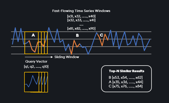
Non-Transformed Temporal Similarity Search offers a dynamic method to search by giving the user the ability to change the number of points to match on runtime – rather than being restricted to a fixed window time. While the search will only return vectors of the same length as the query vector, multiple searches can be run at the same time. This is significant because it allows the matching of various length time vectors simultaneously.
Not only can this similarity search return the top-n most similar vectors, but it can return the bottom-n, or most dissimilar vector. This feature lends itself to outlier detection and is perfect for use-cases where understanding outliers and anomalies is paramount.
Non-Transformed TSS vs. ANN Index: Performance on 1 Million Data Points
To understand the benefits of Non-Transformed Temporal Similarity Search, we compared it to Hierarchical Navigable Small Worlds (HNSW) – an ANN search indexing method – on a dataset of 1 million vectors of 128 dimensions each.
| Non-Transformed TSS | Hierarchical Navigable Small Worlds (HNSW) Index | |
| Memory Footprint | 18.8MB | 2.4GB |
| Time to Build Index | 0s (No Index Required) | 138s |
| Time for Single Similarity Search | 23ms | 1ms (on prebuilt index) |
| Total Time for Single Search (5 neighbors) | 23ms | 138s+1ms |
| Total Time for 1000 searches (5 neighbors) | 8s | 139s |
Non-Transformed Temporal Similarity Search has less than 1% of the memory footprint of an HNSW index for 1 million vectors. Though HNSW has a very fast query time of 1ms, it takes over 2 minutes to build the index in the first place. When accounting for the index build time, Non-Transformed TSS has a total search time 6000x faster for a single query, and 17x faster for 1000 queries.
This performance comparison demonstrates that Non-Transformed Temporal Similarity Search excels for fast moving data where there is not sufficient time to construct an index. In contrast, HNSW or other ANN indexing techniques are more appropriate for static data where there is ample time to construct an index, allowing for speedy searches on the pre-built index.
Non-Transformed TSS Implementation
Getting started with Non-Transformed Temporal Similarity Search is easy, requiring no complex parameters, no need to embed data, and no search index. Querying Non-Transformed Temporal Similarity Search is flexible and can accommodate varied query dimensions to enable diverse data analysis. See the technical documentation for more information.
To create a table in KDB.AI capable of Non-Transformed Temporal Similarity Search, we must define a “tss” vector index type. This example notebook defines a KDB.AI table that will search over fast-moving financial market data vectors.
schema = [
    {"name": "realTime", "type": "datetime64[ns]"},
    {"name": "sym", "type": "str"},
    {"name": "price", "type": "float64s"}
]

# Create the table called "trade_tss"
table = database.create_table("trade_tss", schema = schema)

# Insert data into the table
table.insert(df)

# Perform Non-Transformed TSS Similarity Search
result = table.search(vectors={'price': query_vector}, n=10, type="tss")
In this example schema, we define two metadata columns: “realTime”, and “sym”. We also define a “price” column that where Non-Transformed Temporal Similarity Search will be implemented on time series windows. In for Non-Transformed TSS, we don’t have an index, so there is no need to define an index. Let’s break down the schema and search for understanding:
- Schema column: price – This is the column that will hold the time series window vectors.
- name: price, the name of the column
- type: float64s, the data type of the column
- table.search:
- vectors: specify the column to search on (price), and the query vector
- type: “tss”, Non-Transformed Temporal Similarity Search
- n: The number of top-n results to return from the similarity search.
Non-Transformed TSS Use-Cases
- Financial Market Analysis: Detect trends and identify real-time patterns in stock prices, foreign exchange rates, or trading volumes to forecast market trends.
- Sensor Monitoring: Examine live sensor data from sensors and IoT devices to detect anomalies, predict failures, enhance performance, and power predictive maintenance applications.
- Cybersecurity Threat Detection and Prevention: Monitor unusual network traffic patterns or deviations from standard behavior to mitigate cyber-attack, malware, or unauthorized data exfiltration.
- Healthcare Monitoring: Monitor real-time patient data, including heart rate and blood pressure, to detect health anomalies, predict medical events, and deliver personalized healthcare insights.
Try it Yourself
With Temporal Similarity Search, KDB.AI is empowering developers and business leaders to unveil trends and patterns across diverse and large-scale time series datasets. Whether working with live data or exploring large historical reference datasets, Temporal Similarity Search offers a solution to optimize vector search over your time series data estate.
Check out the documentation to learn more and get started with KDB.AI Temporal Similarity Search.