A practical guide to improving hybrid search performance with hyperparameter tuning.
When incorporating search into your application, it’s tempting to rely solely on the latest advancements in dense embeddings and semantic search. After all, models like BERT and GPT have revolutionized natural language understanding. However, this fascination with dense embeddings often overshadows the enduring power of traditional keyword-based methods like BM25. Surprisingly, in many specialized datasets and real-world applications, sparse search techniques can outperform their dense counterparts. As datasets grow larger and queries become more complex, leveraging the strengths of both traditional and modern search techniques becomes imperative. This is where hybrid search shines, combining the precision of sparse vector search with the contextual understanding of dense embeddings.
But achieving the perfect balance isn’t straightforward. How do we fine-tune the system to maximize retrieval effectiveness? In this article, we’ll dive deep into optimizing the BM25 parameters b and k, and the hybrid search alpha parameter using the HotpotQA dataset. In an in-depth example, I’ll go over how meticulous tuning can significantly enhance search performance — often surpassing methods that rely solely on dense embeddings.
1. Understanding Hybrid Search
Hybrid search combines two powerful approaches to information retrieval:
- Sparse Vector Search (BM25): Relies on term frequency and inverse document frequency to find exact keyword matches. It’s been the backbone of search engines for decades due to its effectiveness in keyword-based retrieval.
- Dense Vector Search (Embeddings): Uses neural network-generated embeddings to capture semantic meaning, enabling the retrieval of contextually similar documents even if exact keywords don’t match.
By blending these methods, hybrid search aims to harness the precision of sparse search and the contextual prowess of dense embeddings.
The Challenge: Balancing these two components effectively. This is controlled by the alpha parameter in hybrid search:
- Alpha = 0: Purely sparse search (BM25).
- Alpha = 1: Purely dense search (embeddings).
- 0 < Alpha < 1: A weighted combination of both.
Our goal is to find the optimal alpha value that maximizes retrieval performance.
2. The Importance of BM25 Parameters
BM25 is a ranking function that scores documents based on their relevance to a query. It introduces two critical parameters:
- k1 (commonly referred to as k): Controls term frequency saturation. It determines how much weight to give to the term frequency in a document.
- b: Adjusts the impact of document length normalization. It balances the importance of shorter versus longer documents.
Fine-tuning b and k is essential because:
- Default values may not be optimal for all datasets.
- Adjusting them can significantly improve retrieval effectiveness, especially in a hybrid search context where BM25 contributes to the sparse component.
It’s worth noting that when we are performing hybrid searches, optimizing b and k is usually much less important than optimizing alpha. There are also other parts of our search pipeline that likely demand more attention, such our reranker, our embedding model, and our data in itself. But depending on our data, tuning b and k can be extremely important!
3. Setting Up the Experiment
To explore the impact of these parameters, we’ll conduct an experiment using the HotpotQA dataset — a challenging benchmark for question-answering systems.
Dependencies
We’ll need the following libraries:
! pip install kdbai_client fastembed datasets ranxImports
import os
import pandas as pd
from collections import Counter
from datasets import load_dataset
from transformers import BertTokenizerFast
from fastembed import TextEmbedding
import numpy as np
import kdbai_client as kdbai
from ranx import Qrels, Run, evaluate
import matplotlib.pyplot as plt
from tqdm import tqdm
4. Preparing the HotpotQA Dataset
4.1. Loading the Data
We start by loading the HotpotQA dataset’s queries, corpus, and relevance judgments (qrels):
# Load the HotpotQA queries, corpus, and qrels (relevance judgments)
queries = load_dataset("BeIR/hotpotqa", 'queries', split='queries[:10000]')
corpus = load_dataset("BeIR/hotpotqa", 'corpus', split='corpus[:10000]')
qrels = load_dataset("BeIR/hotpotqa-qrels")

# Convert qrels to a DataFrame for easier manipulation
qrels_df = pd.DataFrame(qrels['train'])
4.2. Filtering and Aligning Data
To ensure consistency, we filter the datasets to include only overlapping IDs:
# Get the sets of query IDs and corpus IDs
query_ids_set = set(queries['_id'])
corpus_ids_set = set(corpus['_id'])

# Filter qrels to include only IDs present in our queries and corpus
filtered_qrels = qrels_df[
    qrels_df['query-id'].isin(query_ids_set) & qrels_df['corpus-id'].astype(str).isin(corpus_ids_set)
]

# Extract unique IDs after filtering
unique_query_ids = set(filtered_qrels['query-id'])
unique_corpus_ids = set(filtered_qrels['corpus-id'].astype(str))

# Filter corpus and queries based on the filtered IDs
filtered_corpus = corpus.filter(lambda x: x['_id'] in unique_corpus_ids)
filtered_queries = queries.filter(lambda x: x['_id'] in unique_query_ids)
5. Implementing Hybrid Search with KDB.AI
5.1. Initializing Tokenizer and Embedding Model
We use BERT for tokenization and an embedding model for generating dense vectors:
tokenizer = BertTokenizerFast.from_pretrained('bert-base-uncased')
embedding_model = TextEmbedding()
5.2. Preparing Corpus Data
We create both sparse and dense representations for the corpus:
# Extract text and IDs from the corpus
texts = [doc['text'] for doc in filtered_corpus]
doc_ids = [doc['_id'] for doc in filtered_corpus]

# Compute dense embeddings for corpus documents
embeddings_list = list(embedding_model.embed(texts))

# Create sparse vectors for corpus documents
sparse_vectors = []
for text in texts:
    tokens = tokenizer.encode(text, add_special_tokens=False)
    token_counts = dict(Counter(tokens))
    sparse_vectors.append(token_counts)

# Build the DataFrame for corpus data
df = pd.DataFrame({
    'ID': doc_ids,
    'chunk': texts,
    'dense': embeddings_list,
    'sparse': sparse_vectors
})
5.3. Preparing Queries Data
Similarly, we prepare the queries:
# Extract text and IDs from the queries
query_texts = [query['text'] for query in filtered_queries]
query_ids = [query['_id'] for query in filtered_queries]

# Compute dense embeddings for queries
query_embeddings_list = list(embedding_model.embed(query_texts))

# Create sparse vectors for queries
query_sparse_vectors = []
for text in query_texts:
    tokens = tokenizer.encode(text, add_special_tokens=False)
    token_counts = dict(Counter(tokens))
    query_sparse_vectors.append(token_counts)
5.4. Preparing Qrels for Evaluation
We organize the qrels into a dictionary for later use:
# Prepare qrels dictionary for evaluation
qrels_dict = {}
for _, row in filtered_qrels.iterrows():
    query_id = row['query-id']
    corpus_id = str(row['corpus-id'])
    relevance = int(row['score'])
    if query_id not in qrels_dict:
        qrels_dict[query_id] = {}
    qrels_dict[query_id][corpus_id] = relevance
5.5. Setting Up KDB.AI Session
Before we proceed, ensure you have your KDB.AI API key and endpoint ready. You can get a KDB.AI API key and endpoint for free here:
# Set up KDB.AI endpoint and API key
KDBAI_ENDPOINT = os.getenv("KDBAI_ENDPOINT") or input("KDB.AI endpoint: ")
KDBAI_API_KEY = os.getenv("KDBAI_API_KEY") or input("KDB.AI API key: ")

# Start session with KDB.AI
session = kdbai.Session(api_key=KDBAI_API_KEY, endpoint=KDBAI_ENDPOINT)

# Connect to the 'default' database (or another database)
database = session.database('default')
5.6. Defining the Table Schema
We define a schema that includes both sparse and dense vectors:
# Define the table schema
schema = [
    {"name": "ID", "type": "str"},
    {"name": "chunk", "type": "str"},
    {"name": "sparse", "type": "general"},
    {"name": "dense", "type": "float64s"}  # Use float64 for vector embeddings
]

# Define indexes
indexes = [
    {
        "name": "sparseIndex",
        "type": "bm25",
        "params": {"k": 1.25, "b": 0.75},
        "column": "sparse"
    },
    {
        "name": "denseIndex",
        "type": "flat",
        "params": {"dims": len(embeddings_list[0]), "metric": "L2"},  # Adjust dims to match your embeddings
        "column": "dense"
    }
]
5.7. Creating and Populating the Table
We create the table in KDB.AI and insert our data:
import time

# Remove the old table if it exists
try:
    for t in session.database('default').tables:
            if t.name == 'hotpotqa_corpus':
                t.drop()
    time.sleep(5)
except kdbai.KDBAIException:
    pass

table = session.database('default').create_table("hotpotqa_corpus", schema, indexes)

table = session.create_table("hotpotqa_corpus", schema)

# Insert data
table.insert(df)
6. Tuning the Alpha Parameter
Before diving into BM25 parameters, we first need to find the optimal alpha value. This is crucial because alpha dictates the balance between sparse and dense search, and tuning it effectively reduces the search space for b and k.
6.1. Evaluating Different Alpha Values
We evaluate alpha values ranging from 0 to 1 in increments of 0.1:
# Import necessary libraries for evaluation
from ranx import Qrels, Run, evaluate
from tqdm import tqdm  # Progress bar

# Initialize the alpha range (0.0 to 1.0 in steps of 0.1)
alphas = [round(x * 0.1, 1) for x in range(11)]

# Store evaluation results for each alpha
results_by_alpha = {}

# Prepare dense and sparse queries
dense_queries = [emb.tolist() for emb in query_embeddings_list]
sparse_queries = query_sparse_vectors

# Iterate over the alphas and perform batch hybrid search
for alpha in alphas:
    runs_dict = {}
    k = 5  # Number of top documents to retrieve

    # Perform hybrid search with the entire list of queries for the current alpha
    search_results = table.search(
        vectors={
            "sparseIndex": query_sparse_vectors,  # Sparse vector from tokenized queries
            "denseIndex": query_embeddings_list,  # Dense vector from embeddings
        },
        index_params={
            "denseIndex": {
                'weight': alpha  # Weight for dense search
            },
            "sparseIndex": {
                'weight': 1 - alpha  # Weight for sparse search
            }
        },
        n=k  # Number of results to return
    )

    # Iterate over the search results to build the runs_dict
    for i, query_id in enumerate(query_ids):
        runs_dict[query_id] = {}
        for idx, row in search_results[i].iterrows():
            doc_id = row['ID']
            score = row['__nn_distance']  # Use the score returned by KDB.AI
            runs_dict[query_id][doc_id] = score

    # Create Qrels and Run objects
    qrels_ranx = Qrels(qrels_dict)
    run_ranx = Run(runs_dict)

    # Evaluate using ranx
    metrics = ["recall@5", "ndcg@5", "mrr@5"]
    results = evaluate(qrels_ranx, run_ranx, metrics)

    # Store the results for this alpha
    results_by_alpha[alpha] = results
6.2. Visualizing Alpha Tuning Results
We plot the nDCG@5 scores to identify the best alpha:
# Prepare data for plotting
recall_values = [results_by_alpha[alpha]["recall@5"] for alpha in alphas]
ndcg_values = [results_by_alpha[alpha]["ndcg@5"] for alpha in alphas]
mrr_values = [results_by_alpha[alpha]["mrr@5"] for alpha in alphas]

# Plot the results
plt.figure(figsize=(10, 6))
plt.plot(alphas, recall_values, label='Recall@5', marker='o')
plt.plot(alphas, ndcg_values, label='nDCG@5', marker='o')
plt.plot(alphas, mrr_values, label='MRR@5', marker='o')

plt.title('Evaluation Metrics vs Alpha')
plt.xlabel('Alpha')
plt.ylabel('Score')
plt.xticks(alphas)
plt.legend()
plt.grid(True)
plt.show()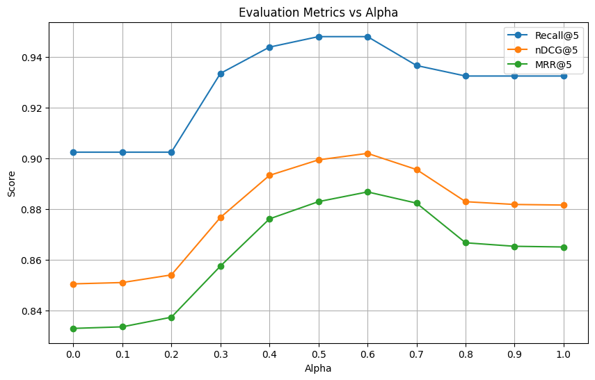
6.3. Determining the Best Alpha
From the plot, we observe that alpha = 0.6 yields the highest nDCG@5 score, indicating the optimal balance between sparse and dense search:
# Find the best alpha based on nDCG@5
best_alpha = max(results_by_alpha, key=lambda a: results_by_alpha[a]["ndcg@5"])
print(f"Best alpha based on nDCG@5: {best_alpha}")
Output:
Best alpha: 0.6 with nDCG@5: 0.5123Insight: This significant improvement over pure sparse (alpha = 0) and pure dense (alpha = 1) search underscores the power of hybrid search when properly balanced.
7. Fine-Tuning BM25 Parameters b and k
With the optimal alpha determined, we can now focus on fine-tuning b and k to enhance the sparse component of our hybrid search.
7.1. Defining Parameter Ranges
We define reasonable ranges for b and k based on their typical values:
# Initialize the range for b and k
b_values = np.arange(0.1, 1.1, 0.2)  # b from 0.1 to 1.0
k_values = np.arange(1.0, 3.1, 0.2)  # k from 1.0 to 3.0

# Store evaluation results for each (b, k) combination
results_by_bk = {}
7.2. Evaluating b and k Combinations
We iterate over all combinations of b and k, keeping the alpha fixed at 0.6:
# Perform batch search for each (b, k) combination
for b in b_values:
    for k in k_values:
        runs_dict = {}
        sparse_index_options = {'b': b, 'k': k}

        search_results = table.search(
            vectors={
                "sparseIndex": query_sparse_vectors,  # Sparse vector from tokenized queries
                "denseIndex": query_embeddings_list,  # Dense vector from embeddings
            },
            index_params={
                "denseIndex": {
                    'weight': best_alpha  # Weight for dense search
                },
                "sparseIndex": {
                    'weight': 1 - best_alpha,  # Weight for sparse search
                    'b': b,
                    'k': k
                }
            },
            n=5,
        )

        # Build the runs_dict
        for i, query_id in enumerate(query_ids):
            runs_dict[query_id] = {}
            for idx, row in search_results[i].iterrows():
                doc_id = row['ID']
                score = row['__nn_distance']  # Use the score returned by KDB.AI
                runs_dict[query_id][doc_id] = score

        # Create Qrels and Run objects
        qrels_ranx = Qrels(qrels_dict)
        run_ranx = Run(runs_dict)

        # Evaluate using ranx (single metric)
        results = evaluate(qrels_ranx, run_ranx, metrics=["ndcg@5"])

        # Since we only have one metric, store the scalar result directly
        results_by_bk[(b, k)] = results
7.3. Reducing the Search Space
By determining the optimal alpha first, we significantly reduce the computational complexity of our parameter tuning. Instead of exploring a vast three-dimensional space (alpha, b, k), we’re now focusing on a two-dimensional grid, making the process more efficient.
8. Analyzing the Results
8.1. Visualizing b and k Impact
We plot nDCG@5 scores against k for each b value:
# Plot nDCG@5 vs k for different values of b
plt.figure(figsize=(10, 6))
for b in b_values:
    ndcg_values = [results_by_bk[(b, k)] for k in k_values]
    plt.plot(k_values, ndcg_values, marker='o', label=f"b = {b:.1f}")

plt.title('nDCG@5 vs k for Different b Values')
plt.xlabel('k')
plt.ylabel('nDCG@5')
plt.legend()
plt.grid(True)
plt.show()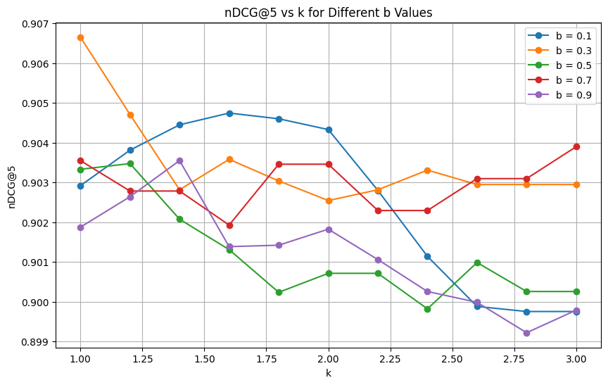
8.2. Finding the Optimal b and k
From the visualization, we can identify the combination of b and k that yields the highest nDCG@5 score:
# Find the best combination based on nDCG@5
best_bk_ndcg = max(results_by_bk, key=lambda bk: results_by_bk[bk])
best_b, best_k = best_bk_ndcg
print(f"Best b and k based on nDCG@5: b = {best_b}, k = {best_k}")
Output:
Best b and k based on nDCG@5: b = 0.30000000000000004, k = 1.0Insight: Fine-tuning b and k after determining the optimal alpha leads to a noticeable improvement in retrieval performance.
9. Key Takeaways
- Hybrid Search Superiority: Combining sparse and dense search methods results in better retrieval performance than using either method alone.
- Alpha Parameter Importance: Tuning the alpha parameter is crucial. In our case, alpha = 0.6 provided the best balance, significantly outperforming pure sparse or dense search.
- Efficiency Through Sequential Tuning: By optimizing alpha first, we reduce the complexity of tuning b and k, making the process more manageable.
- BM25 Parameter Impact: Adjusting b and k further refines the sparse component, leading to additional performance gains.
- Practical Implementation: Incorporating sparse vectors into a vector database like KDB.AI is straightforward, making it practical to implement hybrid search in real-world systems.
10. Conclusion
Through this experiment, we’ve demonstrated the profound impact of carefully tuning hybrid search parameters. By first identifying the optimal alpha value, we effectively balanced the contributions of sparse and dense search methods. Subsequently, fine-tuning the BM25 parameters b and k allowed us to extract even more performance from the sparse component.
In this particular example, optimizing b and k parameters gave us an insignificant performance boost, and the KDB.AI defaults would have been sufficient. Typically, it makes more sense to optimize other parts of the search pipeline, including our chunking, embedding, alpha choice, and reranking strategy before even looking at b and k! But our alpha choice made a massive difference, improving ndcg by around 5 points. A good place to start is an alpha of .5 to .7 for non domain-specific texts, and .3 to .5 for very domain-specific, technical texts such as legal or medical documents. For our dataset, .6 was the ideal alpha parameter, but .5 would have performed pretty much the same.
It’s also worth noting that we don’t need to use BM25 for our sparse index. We can just as easily use SPLADE or other sparse embeddings, which might outperform BM25 in some cases. When using sparse embedding models besides BM25, tuning hyperparameters becomes even more important, as other sparse encoders may not have as established guidelines as BM25.
Final Thoughts: In an era where dense embeddings are gaining popularity, it’s essential not to overlook the enduring strengths of traditional methods like BM25. Hybrid search, when optimized, leverages the best of both worlds, delivering superior retrieval results.