Vector databases utilize a crucial element known as the “Vector Index” to process data. The creation of this index involves applying an algorithm to the vector embeddings stored within the database. This algorithm functions to map these vectors to a specialized data structure, facilitating rapid searches. Searches are more efficient this way due to the index’s condensed representation of the original vector data. This compactness reduces memory requirements and enhances accessibility when contrasted with processing searches via raw embeddings.
You don’t need to know the details of creating indices themselves with KDB.AI; they are easily created through simple commands that you choose. However, grasping the fundamental workings of vector indices and their various forms can be helpful in knowing which one to choose and when. This article discusses three primary categories of vector indices:
- Flat (e.g. Brute Force)
- Graph (e.g. HNSW)
- Inverted (e.g. IVF, IVF-PQ)
Flat Index
Flat indices (otherwise known as “Brute Force”) deliver the best accuracy of all indexing methods, however, they are notoriously slow. This is because flat indices are a direct representation of the vector embedding. Unlike other indexing methods, generating flat indices does not use pre-trained clusters or any other modification of the vector embeddings. With flat indices, search is exhaustive: it’s performed from the query vector across every single vector embedding and distances are calculated for each pair. Then, k number of embeddings are returned using k-nearest neighbors (kNN) search:
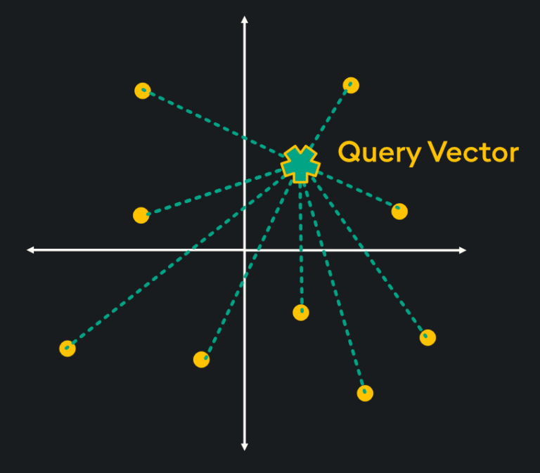
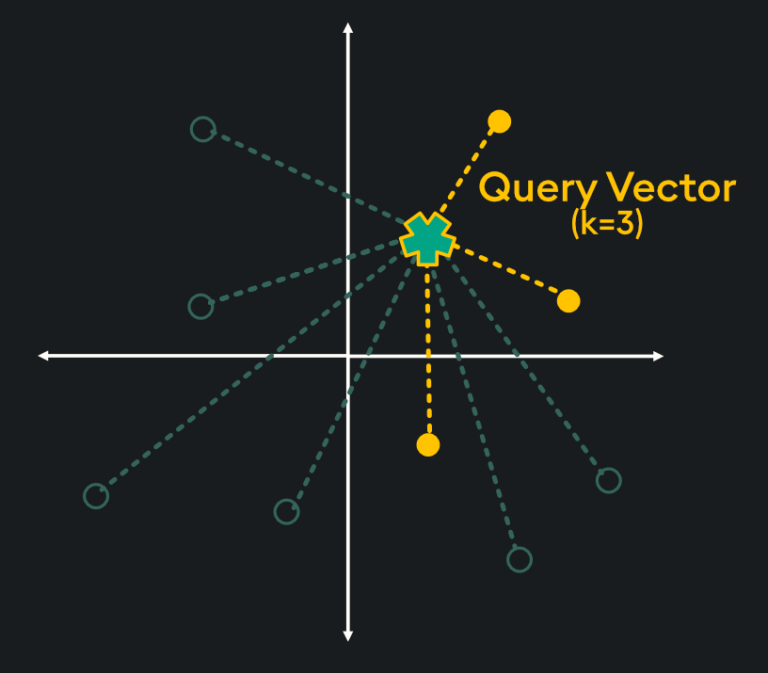
This type of pairwise distance calculation doesn’t seem very efficient (hint: it’s not), however, the high accuracy of search results is sometimes required depending on your application. Specifically, here are some scenarios in which flat indexing is beneficial:
- Low-Dimensional Data: With low-dimensional vectors, typically up to a few dozen dimensions, flat indices can be sufficiently fast while maintaining high accuracy.
- Small-Scale Databases: When the database contains a relatively small number of vectors, a flat index can be sufficient to provide quick retrieval times.
- Simple Querying: If the primary use case involves simple queries, a flat index can offer competitive performance compared to other indices without the complexity.
- Real-time Data Ingestion: When vectors are continuously added to the database, they must be indexed quickly. Due to the simplicity of flat indexing, minimal computation is needed to generate the new indices.
- Low Query Volume: If the rate of queries being performed on the database is low, a flat index can handle these queries effectively.
- Benchmarking Comparisons: In situations where you want to evaluate the accuracy of other index methods, using the perfectly accurate flat index can be used as a benchmark for comparison purposes.
qFlat
The qFlat index introduces a novel approach to vector indexing by storing the index on-disk rather than in-memory. This enables substantial improvements in resource utilization while maintaining the accuracy benefits of flat indices.
Similarly to flat indices, qFlat is a great choice for datasets of up to 1,000,000 vectors where accuracy is paramount. The primary goal of qFlat is to provide a vector index option that is not constrained by memory limitations. As long as there is enough disk space available to store your dataset, the index can be searched.
With the qFlat index, data ingest is high speed with negligible memory and CPU footprint, and search is read from disk incrementally, maintaining very low memory utilization.
Assumptions
- Disk Storage Access: Access to disk storage is required for the qFlat index to function.
- Impact of Disk Speeds: The speed of disk storage will have a direct impact on search performance, making faster disks preferable for optimal performance.
Overall, the qFlat index offers a memory-efficient solution for vector indexing and is particularly useful in memory constrained environments, for example edge devices.
Graph Indexes (HNSW & qHNSW)
Graph indices use nodes and edges to construct a network-like structure. The nodes (or “vertices”) represent the vector embeddings while the edges represent the relationships between embeddings. The most common type of graph index is Hierarchical Navigable Small Words (HNSW).
HNSW is a “proximity graph” where two embedding vertices are linked based on their proximity – often defined by Euclidean Distance. Each vertex in the graph connects to other vertices called “friends” and each vertex keeps a “friends list.” Starting at a predefined “entry point”, the algorithm traverses connected friend vertices until it finds the nearest neighbor to the query vector:
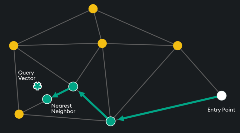
Each traversal is continued on via Nearest Neighboring vertices in the “friends list” until no nearer vertex is found – a local minimum is reached for distance.
The entry point is typically on high-degree vertices (vertices with many connections) to reduce the chance of stopping early by starting on low-degree vertices:
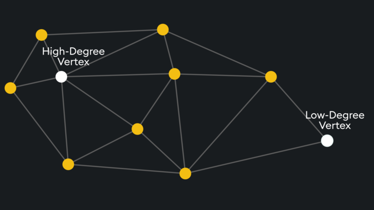
The number of degrees on the entry vertex can be specified and is typically balanced between recall and search speed.
Rather than doing this across one layer (which would take considerable time and memory), the index space is split into hierarchical layers, thus the “H” in HNSW:
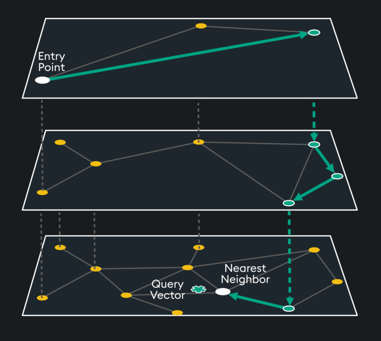
The top layer has the longest distances but includes the highest degree vertices. The algorithm starts by traversing the longer distances until it finds a local minimum with the high degree vertices, then it drops down a layer where more “friend” vertices are available to the previous layer’s high degree vertex. This traversal continues until the nearest neighbor’s distance to the query vector reaches a local minimum.
KDB.AI offers two versions of HNSW, traditional in-memory HNSW, and an on-disk version called qHNSW. While HNSW stores all data in-memory, qHNSW addresses this limitation by allowing for on-disk storage with memory-mapped access. The result is qHNSW is a more scalable and efficient indexing solution (especially for memory constrained environments) that can handle large datasets without being bound by available memory.
Specifically, here are the scenarios where HNSW / qHNSW indexing makes the most sense:
- High-Dimensional Data: HNSW is specifically designed for high-dimensional data, typically hundreds or thousands of dimensions.
- Efficient Nearest Neighbor Search: HNSW is well-suited for applications where quickly finding the most similar data points to a given query is critical, such as recommendation systems, content-based image retrieval, and natural language processing tasks.
- Approximate Nearest Neighbor Search: While HNSW is primarily designed for accurate nearest neighbor search, it can also be used for approximate nearest neighbor search tasks where the user seeks to minimize search computation cost.
- Large-Scale Databases: HNSW is designed to scale well with large datasets.
- Real-time and Dynamic Data: HNSW is capable of accommodating dynamically changing data, such as real-time updates.
- Highly-Resourced Environments: HNSW’s performance is not solely reliant on the memory of a single machine, making it well-suited to distributed and parallel computing environments.
Inverted Index (and Product Quantization)
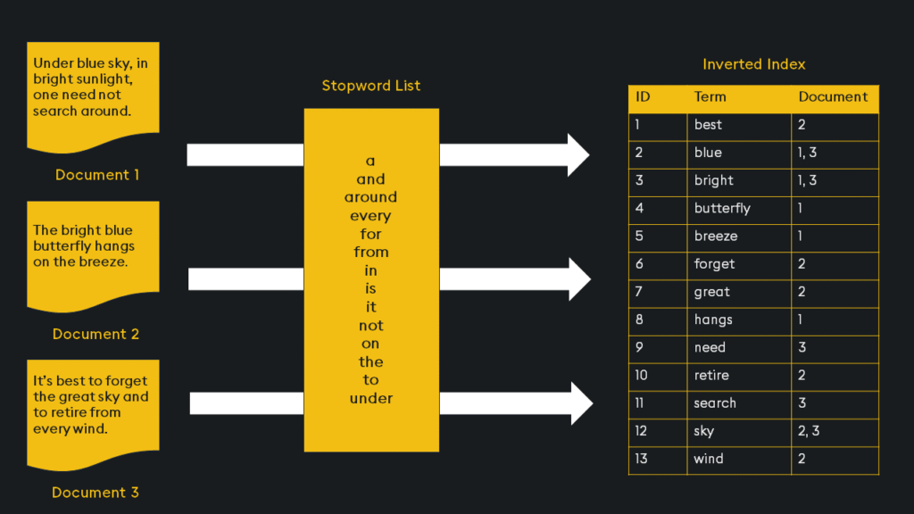
Inverted indices are widely used in search engines because they provide an efficient way to find document contents. Imagine you have a collection of documents, like web pages in a search engine database. Each document contains words, and you want to be able to quickly find all the documents that contain a particular word. For each unique word in the entire collection of documents, the inverted index creates a list of document references or identifiers (such as document IDs) where that word appears:
This is an initial broad stroke of the indexing. We can further optimize the index with “Product Quantization”.
Product Quantization works in 4 steps:
- Take a high dimensional vector
- Split into equally sized sub-vectors
- Assign each subvector to its nearest centroid (defined by kmeans clustering)
- Replace each centroid value with Unique IDs
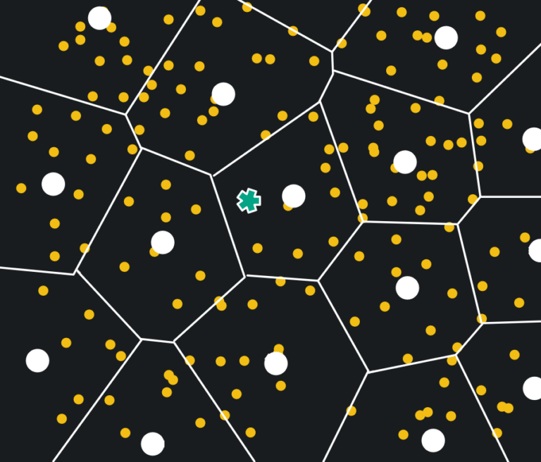
Once the quantized subvectors are available, they can be arranged in Voronoi cells. This is shown below with subvectors in yellow, Voronoi cells bounded by white lines, and their centroids in white circles. The query vector is the green star:
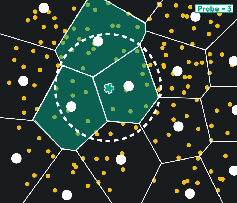
The Voronoi cells chosen are defined by the query vector and probe parameter. Search is restricted to the cell the query vector lies in, and nearest centroids of surrounding cells. Below, a probe parameter of 3 grabs the 3 nearest cells to the query vector:
This yields a huge reduction in memory usage and search time, with great recall. Like HNSW, it’s well-suited to high dimensional vectors and when you need fast nearest neighbor search. In fact, IVFPQ shares a lot of similar benefits as HNSW ranging from Highly-Resourced Environments, to High-Dimensionality Vectors, to Large-Scale Databases. It would be more useful to highlight the nuanced differences in the two index types:
IVFPQ Index is better for:
- Accuracy: Excels when high precision of nearest neighbors is important.
- Approximate Search: Both exact and approximate nearest neighbor search are used, however, it’s particularly strong in scenarios where exact results are desired.
- Memory Efficiency: Due to the use of product quantization, IVFPQ is very memory efficient.
HNSW Index is better for:
- Approximate Search: HNSW is designed for efficient approximate nearest neighbor calculations. If your goal is to find a relatively good solution quickly, even if it’s not the exact nearest neighbor, choose HNSW.
- Simplicity: HNSW is relatively simpler to implement and configure compared to IVFPQ. There are fewer steps in constructing the index since PQ is not involved.
- Scalability: Handles large datasets with ease and is adaptive to real-time and dynamic data.
- Storage: HNSW does not require PQ, and therefore needs less storage space.
- Speed (over accuracy): If you can accept approximate results, the speed benefits of HNSW may be worth it.
Final Considerations
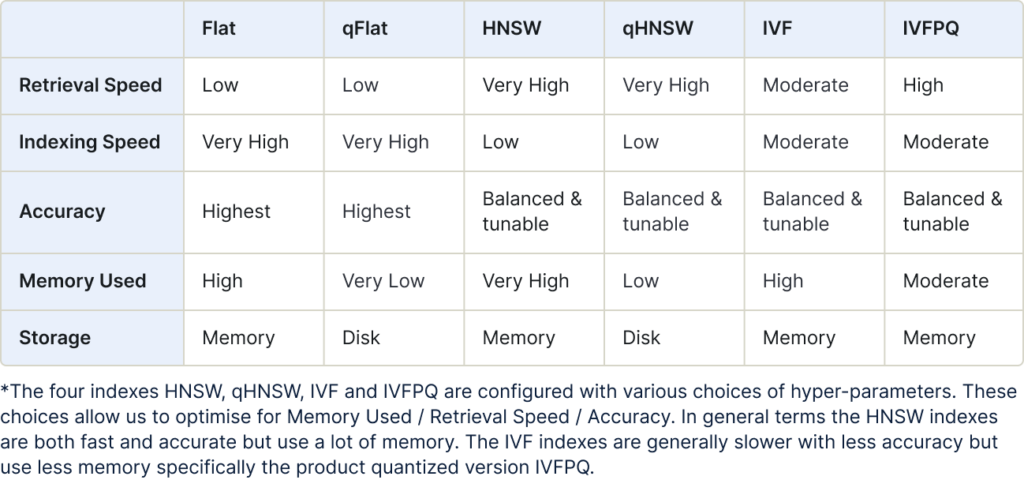
The benefits of each index type described here can be summarized in the following table:
Compare All Indexes
The benefits of each index type is summarized in the following table:
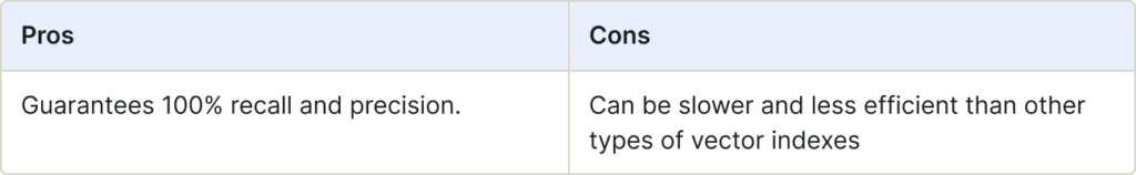
Flat Index
Also known as “Brute Force,” Flat indexes offer a straightforward approach that involves comparing vectors directly, making it suitable for smaller datasets.
Flat indexes are stored in-memory, while qFlat indexes are stored on-disk.
Use for:
- Low-dimensional data
- Small-scale databases
- Simple querying
- Real-time data ingestion
- Low-query volume
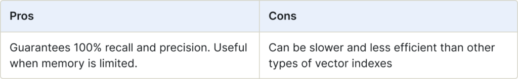
qFlat Index
The qFlat search performs an exhaustive search against all vectors in the search space. You can configure it with a number of distance metrics. As the search is exhaustive, it finds the exact nearest neighbors without approximations.
qFlat indexes are stored on-disk, while Flat indexes are stored in-memory.
Use for:
- Situations when you would use Flat, but memory is limited
- Low-dimensional data
- Small-scale databases
- Simple querying
- Real-time data ingestion
- Low-query volume
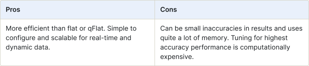
HNSW (Graph Index)
Hierarchical Navigable Small Worlds (HNSW) is a graph-based index that organizes vectors in a graph structure and navigates through the graph to find approximate nearest neighbors. HNSW is suitable for large-scale databases with moderate accuracy requirements.
HNSW indexes are stored in-memory, while qHNSW indexes are stored on-disk.
Use for:
- Medium-Large scale datasets
- Good accuracy
- High-dimensional data (hundred or thousands of dimensions)
- Efficient nearest neighbor search for
- recommendation systems
- content-based image retrieval
- NLP tasks
- Approximate nearest neighbor search when looking for cost reduction
- Large-scale databases
- Real-time and dynamic data
- Highly resourced environments (distributed and parallel computing)
qHNSW (Graph Index)
The q Hierarchical Navigable Small Worlds (qHNSW) index establishes connections between vertices in the graph based on their distances. This approach is extremely efficient with search performance a measure of the complexity of the graph.
qHNSW indexes are stored on-disk, while HNSW indexes are stored in-memory.
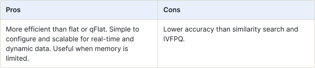
Use for:
- Situations when you would use HNSW, but memory is limited
- Medium-Large scale datasets
- Good accuracy
- High-dimensional data (hundred or thousands of dimensions)
- Efficient nearest neighbor search for
- recommendation systems
- content-based image retrieval
- NLP tasks
- Approximate nearest neighbor search when looking for cost reduction
- Large-scale databases
- Real-time and dynamic data
- Highly resourced environments (distributed and parallel computing)
IVF (Inverted Index)
Inverted File (IVF) is an efficient data structure used for approximate nearest neighbor search. It helps narrow down the scope of vectors during search, significantly improving search speed. IVF maps contents (vectors) to their locations, making it easier to retrieve relevant information from large datasets.
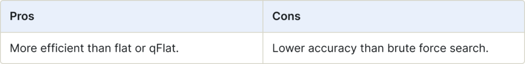
Use for:
- Large-scale datasets
- High-dimensional data (hundred or thousands of dimensions)
- Fast searches
IVFPQ (Inverted Index)
IVFPQ combines IVF (Inverted Index) with Product Quantization (PQ). PQ is a technique for dimensionality reduction without losing essential information. Initially, IVF narrows down the search scope by using an inverted file index. Next, PQ further compresses the vectors, allowing efficient search with a reduced number of vectors.
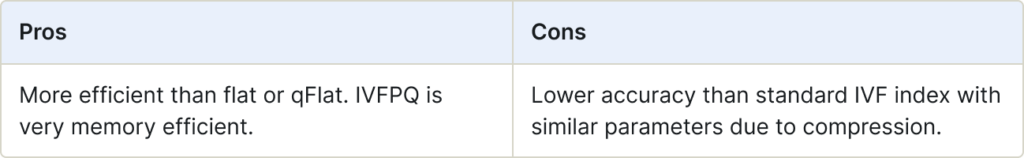
Use for:
- Large-scale datasets
- Situations where accuracy is not critical
- Memory efficiency
It’s important to remember that KDB.AI does vector indexing for you through simple commands, however, this article covered some important considerations and inner workings of how those indices are created as well as the specific tradeoffs to help you better decide how to use them.
To index your own vector embeddings, read our documentation.