Semantic search has introduced a revolutionary new mode of information access. Instead of having to search by keywords (e.g. Google), you can now find information based on meaning. This might sound trivial but it’s not. It allows higher quality search results that can then be used for a variety of new applications, such as language generation, search engine optimization, and more. To fully understand semantic search, it’s recommended you understand Vector Indexing Basics and Methods of Similarity Search. In general, the full process of searching across vector embeddings is as follows:
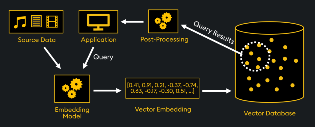
- Generate Vector Embeddings of Source Data
- Index those Embeddings
- Process Queries from your Application
- Perform Similarity Calculations
- Rank and Retrieve Query Results
- Post Processing of Retrievals
Since the first two bullet points are covered in our articles on Vector Embeddings and Vector Indexing Basics, this article focuses on the last four bullet points, pertaining more to the search itself.
Processing Queries
The first step to search is to process the queries into the same vector space as the database. For text-based search, this means that plain human text needs to be converted into the same format as the embeddings themselves:
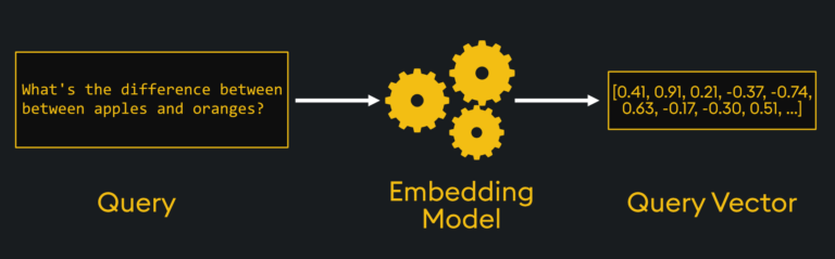
The process involves creating a “query vector.” This is generated from the input text, processing it through your embedding model (and any other feature engineering steps also applied to your other embeddings), and finally creating a query vector that lands in the appropriate part of the vector space. Other than text as an input, code, images, video, audio and other formats can be used, but all will still generate a numerical arrayed query vector.
The query vector should be generated using the same embedding model that was used to generate your content embeddings stored in the database. This is important because you need to map existing content in the same embedding format as your query, in the same vector space, to perform similarity calculations.
Similarity Calculations
The query vector will land in the vector space of your other embeddings. Below, for a 2-dimensional vector space, the query vector is the green star while the other embeddings are yellow circles:

From there, the nearby vectors are identified and returned, which is done by any one of a variety of methods. A few common examples are brute force (i.e. “exact”) search, k-Nearest Neighbors (KNN) search, and Approximate Nearest Neighbor (ANN) search. Within these search types, there are specific methods of indexing for retrieval such as flat index, inverted index, and graph index, which are all covered in our Vector Indexing article.
Note the vector indexing is performed prior to the search, but the similarity calculation is performed during the search. Common similarity metrics include Euclidean Distance, Dot Product, and Cosine Similarity, explained in our Methods of Vector Similarity article. You may choose which similarity metric you would like to use with your indexed search. Optimal similarity types for different applications are detailed in the article.
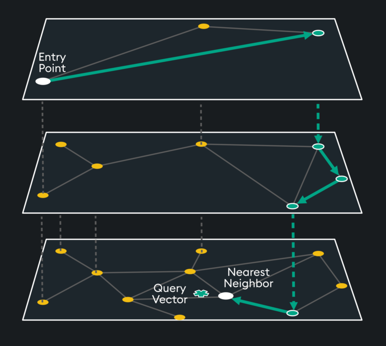
As an example, a fast search method used by KDB.AI is Hierarchical Navigable Small Worlds (HNSW), a type of ANN search using a graph index. There are multiple layers of indexed embeddings of increasing granularity. The query vector is placed at the bottom layer while the entry point for search is the top layer. The search traverses nearest neighbors of a graph index, until it finds the local minimum at each layer of the index. When it gets to the local minimum of the final layer, it is done with the search.
Ranking and Retrieval
Okay, so which vector embeddings are actually returned? This depends on the ranking and retrieval you have set up. Typically, once the similarity scores are calculated between the embeddings and the query vector, they are then ranked in descending order of similarity. This ensures the most relevant search results are at the top of the list.
Depending on the application, the entire ranked list may be returned, or only the top-k results (where k is predefined by the system requirements or user’s preferences). Retrieval systems can also incorporate user interaction and feedback to further personalize results. Feedback mechanisms like relevance feedback data can be used to adapt the ranking and improve relevance of search results over time.
Post Processing
Post processing actions may be taken after the query results are retrieved. They include operations such as Ranking Refinement, Deduplication, Filtering, Clustering, Personalization, and more. Let’s discuss some applications of a few of these:
- Ranking Refinement: recommendation systems, like e-commerce platforms, rank results of a search that are most relevant to a user’s query.
- Filtering: in search engine results, items with very low similarity scores can be excluded from the overall results.
- Clustering: in anomaly detection, search results that deviate from typical data patterns defined by clusters can be returned to the user.
- Personalization: by factoring in users’ listening history on music platforms, search results can better align with the users’ taste preferences.
- Deduplication: when integrating data from multiple data warehouses, deduplicating search results eliminates duplicated records.
Post-processing techniques can significantly impact the quality and relevance of search results. However, the specific post-processing methods used will depend on the application, the characteristics of the data, and the user’s information needs.
Making Vector Search Work for You
In conclusion, you must first have vector embeddings of your content in your vector database which a query vector is then used with similarity search to find similar content. Results are ranked and retrieved, then post processing is performed to optimize the relevance of retrieved content. To get started with your own vector search, visit our documentation.